 In the last lesson I showed you how to select and copy a column of data from one spreadsheet to another. In this lesson, I’ll go into more ways to copy data in Excel by copying and pasting multiple columns. I also show with how to paste data into a new column of an existing spreadsheet. To complete this lesson, you need to create a work tab as instructed in Part 1.
Selecting Multiple Columns to Copy Data in Excel
Click on the first column of the group of columns you want to copy. In the example, I started with Column C, Name. While holding down the mouse button, scroll over the columns to one you want to end with. I ended with Column G, Type.

With the columns highlighted, right-click to bring up the menu and select Copy.

Click on the Work Tab and press Enter. As seen in the following example, the columns have been copied into the Work tab.

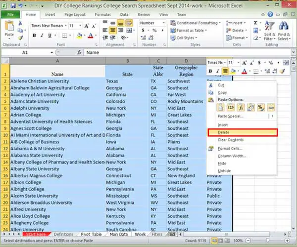
Delete the columns with data in the Work tab so that we can use it for another example. Highlight the Columns A to E, right click, and select Delete from the menu.

Understand Space Requirements When You Copy Data in Excel
Return to the Filters tab. The data in the Filters tab should still be highlighted. Over the highlighted area, right-click and select Copy again. Then go to the Work tab and select the cell C3. Right click and select the Paste icon.

When you pasted, you saw the following message:
This happened because the area copied was the entire column. Because I selected some place other than the top of the column or the top cell in the column, Excel couldn’t fit the entire column. When I select the first cell of Column F, Excel pastes the information.

If you selected just the data using the extended selection method discussed in the last lesson, this wouldn’t happen as long as there were enough rows to accommodate the data. The same thing happens if you select entire rows to copy and then don’t start the paste in the A column.
You don’t need to highlight the entire area where you want to paste something. As long as there is room, Excel will paste the data. You just need to select the upper-left hand cell of the area you want to paste.
Delete to data columns as before for the next step.
Copying Non-adjacent Columns
What if I want to copy columns not next to each other? For example, I want to copy the Name, State Abbr, and Type columns.
Start with the Name column, column C. Select the column while holding down the control key. While continuing to hold down the key, select the E column, State Abbr, and Column G, Type.

Right click for the menu and select Copy. Click on the Work tab and press enter (or right click and select the Paste icon).

Notice that Excel pasted all three columns next to each other. There are no columns in-between. You can do the same thing with rows. Delete the columns with data from the work tab.
When working with big spreadsheets, sometimes the columns you want to paste are far apart. While you’re scrolling to select the columns, it’s easy to lift your finger off the control key. One thing you can do is to hide the columns (see the lesson on Spreadsheet Geography) so that the columns you want to select are altogether.
I’m going to repeat the previous example. This time I’ll hide the State column D and the Geographic Region column F. It’s tempting to just highlight the 3 columns as you would with a regular selection, clicking on the c column and moving the cursor. You can do this but Excel is going to copy all of the columns, including the hidden ones.
You can see the difference when you first select the columns. Excel highlights the columns individually when you use the control key

The following shows a selection made just by scrolling to select the columns.

The only reason there are internal selection lines in the above example is because the selection includes frozen rows and columns. Go ahead and copy the Name, State abbr, and Type columns to the Work tab.
Inserting Copied Cells
Go back to the filters tab. I’m going to scroll over to column BI and select the SAT/ACT Required column. You can pick any column that you prefer for this example.

Copy the selection and then click on the Work tab. I want to paste the SAT/ACT information between the A and C column. In ancient times, this would have required that I insert a blank column and then copy and paste the data. No longer.
Select the State Abbr column in the Work tab. Right click and select Insert Copied Cells.

Excel inserts a new column and pastes the information copied from the Filters tab.

This is why it’s referred to as an “Insert” copy. You aren’t pasting into an existing column. This can be a very useful way for moving data. Delete the work tab to finish this lesson.
There’s much more to come on how to copy data in Excel. But before I go any further, I think I need to talk a little about data formatting and formulas. So in the next lesson I’ll show you some of the ways Excel allows you create and format data.


2 thoughts on “Creating College Lists 101: Copying Data-Part 2”