 I’m going to take a break from showing you how to copy data so that I can go over some of the ways of formatting data in Excel–including by copying. Excel provides more ways to format data than any one person could ever need. So I want to begin by showing some basic formatting options that I use frequently when creating my college lists.
For this lesson, I’m going to be working with an empty spreadsheet. You can create a new file or just create a new worksheet tab in an existing workbook.
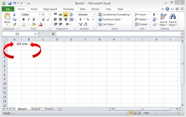
In the A1 cell, enter 123. In the cell next to it, B1, enter the word one. Your spreadsheet should look like the one below:
Notice that the number is aligned to the right side of the cell while the text is aligned to the left. These are the default alignments for numbers and text in Excel.
Formatting Numbers
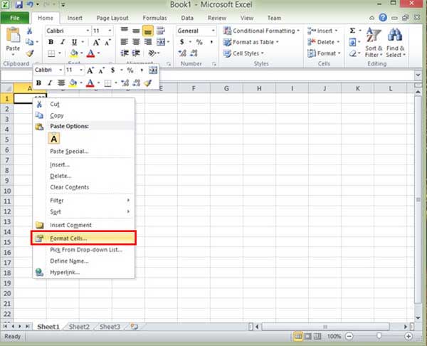
Select the A1 cell with the number. Right click and select Format Cells from the menu.
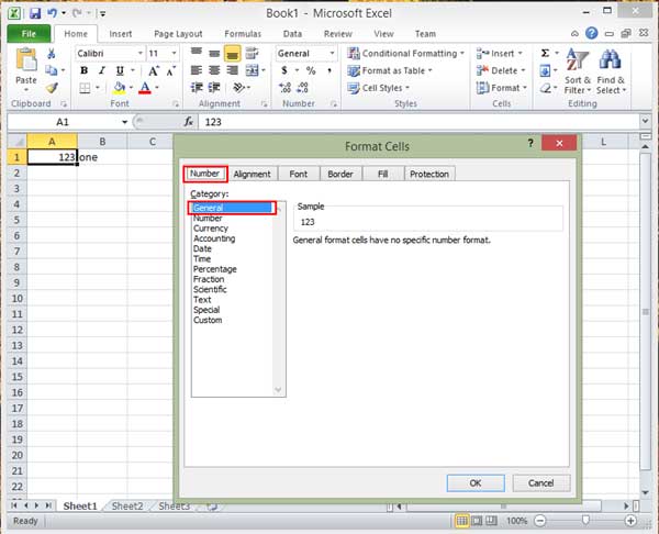
This will bring up the Excel Format Cells Dialog box. Under the Number tab, you see that the cell is formatted as General which is the default.
Change the Category from General to Number. Set the number of Decimal places to 1 and check the Use 1000 Separator box. As you make your selections, Excel will show you what the number will look like in the Sample box.
Click the OK button to save your changes. The number now has a decimal point followed by a 0. You don’t see the thousand separator because the number isn’t large enough.
In cell C1, enter the number 9876.
Return to cell A1 and bring up the menu by right clicking. Select Copy.
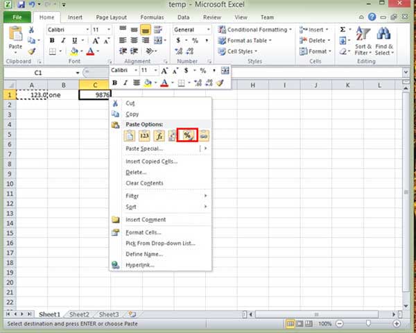
Now select cell C1 and right-click to bring up the menu. Under the Paste Options select the Format icon.
This option copies just the formatting, not any of the values. The number is now formatted with a thousand separator and one decimal place just as I had set it for the cell A1.
Wrapping Text
Excel allows you to control the alignment and have text wrap as needed. Select cell B1, right-click, and select Format Cell to bring up the Format Cell dialog box. Click on the Alignment Tab. Under the Text Control options, check the Wrap text box.
Click the OK button to save your changes. Since the text one doesn’t exceed the length of the cell, you don’t see any differences.
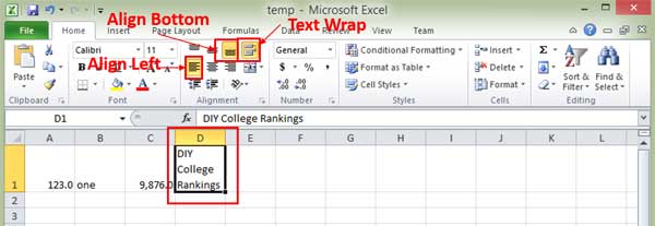
Enter DIY College Rankings in the D1 cell. You’ll see that the text extends beyond the boundaries of the cell. If the E1 cell contained information, the text in cell D1 would appear truncated. The cell would still contain all of the information, Excel just wouldn’t be able to show it.
Move the cursor to the B1 cell and copy the information. Next, move back the D1 cell and paste only the formatting to the cell as in the previous example. The text in the cell will now wrap, increasing the row height to accommodate the text.
Notice on the Home tab ribbon, several icons in the Alignment section are highlighted in yellow. These indicate the formatting currently applied to the selected cell–in this case, Align Left, Align Bottom, and Text Wrap.
Many of the options for formatting data in Excel that you can access through the right click menu are available on the ribbon as well. Where you choose to access the options is a matter of personal preference.
Centering and Merging Cells
When creating a table, you often want a title to actually expand across several columns of information. Again, this is something you can do easily in Excel.
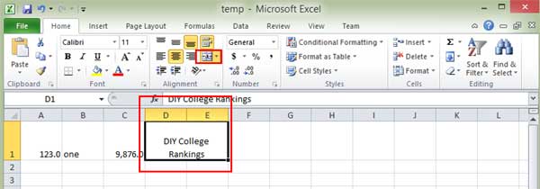
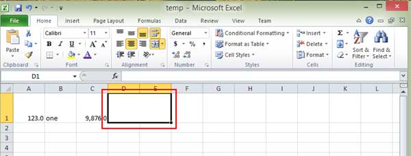
In the example, I want the text DIY College Rankings to appear in the D and E cells. To do this, select both the D1 and E1 cells as in the example.

Instead of right clicking for the menu, click on the dropdown arrow by the Merge icon in the Alignment section of the Home ribbon. Then select the Merge & Center option.
Excel combines the two cells and centers the text. Since the merged cells still aren’t big enough, the text is still wrapped.
During all of the lessons so far when I right-click to bring up menu options, I have been referring to the long menu with a list of options. However, if you’ve been paying attention you’ll have noticed that there is actually another menu that appears as well. This is a menu of icon options that appears above the text option we’ve been using. This menu is a great shortcut for many formatting options.
Changing Color
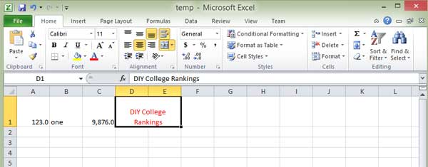
Click on the DIY College Rankings cell and then right click to bring up your menu options. In the top menu click on the Letter A with the red underline to change the font color to red.
The text is now red. If you had selected the dropdown arrow by the letter A, you could have picked a different color.
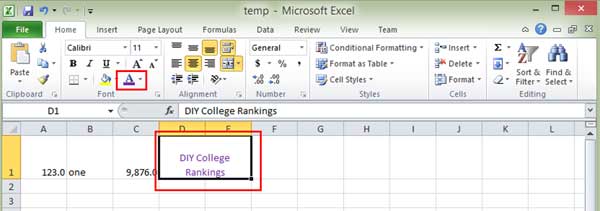
You can also change the color using options on the Home ribbon. With the cell highlighted, click on the arrow by the letter A with the red underline in the Font section.
This will bring up a color palette menu of choices. Pick some color other than red, I chose purple.
You’ll see that the red line under the letter A has changed to the color you selected, in my case purple. You’ll also see the various formats applied to the current cell in the Alignment section of the ribbon including the highlighted Merge Icon.
Formatting Row Height
You may have noticed that when you centered and merged the DIY College Rankings text, the text wrapped to only two lines instead of the three it had in just one cell. However, the row height remained the same so there is some white space above the text. Go ahead and delete the DIY College Rankings text completely.
Now click on row number 1 to select the entire first row. Then click on the arrow for the Format Icon in the Cells section of the Ribbon. Select AutoFit Row Height.
Excel adjusts the height of the row to fit the tallest contents automatically. I use this option rather than adjusting the height myself by dragging on the row dividing lines.
You can do the same thing with column widths.
I know this has been a smorgasbord of ways of formatting data in Excel. My intent was to show you how to use the right-click menu or the ribbon menu to access the various options. You don’t have to actually click on the ribbon icons to see what they do. If you hover over an icon, an information box will appear with a brief explanation of what the icon does.
This can be a useful way to discover useful features you didn’t even know existed. In the next lesson I’ll show some ways to calculate the data.









1 thought on “Creating College Lists 101: Introduction to Formatting Data in Excel”