 Sooner or later while you’re looking at the data for a specific college, you’re going to wonder if a certain number is a good thing or a bad thing? It’s at this point you realize it would be good to know the average SAT scores for the schools you’re looking at. Or maybe what are the highest and lowest graduation rates. It would help you put an individual school’s number in context. So this week, I’m going to do an introduction to calculating data in Excel.
This lesson is going to draw on topics covered previously including copying data and using filters. In other words, I’m not going to tell you how to copy data step by step, I’m just going to give it as a direction. If you need help, check out the earlier lessons.
We’Il begin by inserting a new blank worksheet. In the example, I’m just sticking with the default name Sheet 1.
To show you how to perform data calculations, we need some data. In the DIY College Rankings Spreadsheet, go to the Filters tab and select all the schools in Maine. This provides a small number of schools to work with.
Copy the Name, Full-time Undergraduates, and 4/5 Year Grad Rate columns to Sheet 1. You don’t actually need the names for this lesson. I just find that even with examples, there will be times you want to know where a certain number comes from and this way you’ll have the school name right here.
Calculating Totals
Select the data from the Full-time undergraduates column. While not a big deal here, remember that you can click on F8 which activates Excel’s Extend Selection and allows you to just click on the Control and down arrow keys simultaneously to select all of the data in the column.
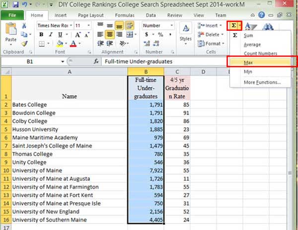
What we want to do is to total the number of Full-time undergraduates. While the data is highlighted, select the Sum Icon Menu from the Home Ribbon. From the dropdown menu, select the Sum option
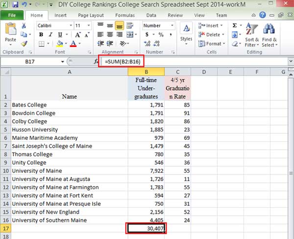
Excel calculates the total for the column and inserts it in the cell immediately below the last cell of data. According to this calculation, there are 30,407 full-time undergraduates in Maine.
If you look on the status bar at the bottom, you’ll that Excel provides some summary information for the selected data.
You’ll notice the Sum is twice that of what is in cell B17 since the calculated total is part of the data selection.
Select the cell that is displaying the total. In the example it’s cell B17 with the value 30,407. If you look in the formula bar, you’ll see the formula Excel used to total the data.
The formula starts with an = sign. This is how you tell Excel you’re entering a formula. If you just enter “2+2” into a cell, all you will see is “2+2.” You need to enter =2+2 to have Excel add the numbers.
Copying Formulas
Select the cell with the total formula, B17, and copy it to C17.
Excel automatically adjusts the formula so that it now shows the sum for column C. This means that when you copy formulas, the location of the cells are relational.
In the example, Excel assumes that when copy the formula to column C, you really don’t want the total for column B. You want the formula to sum whatever data is immediately above it. So Excel changes the column from B to C when you copy the formula.
Go ahead and copy the original total cell, B17, again. This time when you paste in the neighboring cell, C17, select the Values Only option-the 123 menu icon.
This time, Excel pasted the value from the calculation, 30,407–not the formula used. If it was the formula, you would see it in the formula bar and the total would be 725.
Why would you need to do this? Because as you select and compile data for use, you want to work with the actual values. If you copy the formulas, you’re likely to generate errors or the wrong value because Excel is automatically adjusting the formula so that it is relative to where you paste it.
Often after I have set up a table that includes data calculations, I copy entire table and then paste it over itself with the values only option. This eliminates all of the formulas leaving only actual values to copy in the future.
Select the B17 and C17 cells and click Delete.
Find the Max Value
Select all of the data from the Full-time Undergraduates as we did earlier. This time, select the Max option from the Sum Menu.
Excel displays the highest value at the bottom of the select cells, In the example, the greatest number of Full-time Undergraduates was 7,922 at the University of Maine, which is the value Excel displays.
Subtracting Data in Excel
We’re going to create a third column of data. Enter Difference in cell D1 as the title for the column. In cell D2, enter the formula =B2-C2.
You don’t have to enter the actual cell addresses when entering a formula. The larger your spreadsheet gets, the more likely you are to enter an address incorrectly. What you can do instead of entering the actual cell address is to click on the cell you want to use. Excel will outline the selected cells in Blue.
You end up with the same results. It’s just a different way of entering the same formula.
Now we want to copy this formula for the rest of the column. We could do a copy and paste since it’s such a short column. However, when dealing with longer columns, you might find it easier to hover the mouse over the lower right-hand corner of the cell with the formula until a plus sign appears. Once you see the plus sign, double click and Excel will copy and paste the cell contents down the rest of the column.
 Relative Addressing
Next we’re going to take a closer look at the relative addressing properties of the formula. Let’s say we want the numbers in columns C and D represented as percentages of column B. These numbers are totally meaningless. The point is that whatever formulas we enter in columns E and F should combine for a total of 100%.
In the example, I added two more column titles Division 1 and Division 2 since that is what we’re going to be doing. In the E2 column, enter the formula =C2/B2.
Let’s go ahead and format it as a percentage. Select the % Menu Icon from the Home Ribbon’s Number section.
Excel automatically formats the number as a percentage as seen in the following example.
Now copy the formula from E2 to F2.
The fact that the value is 2007% is a hint that the percentages aren’t adding up to 100 as they should. The problem is that Excel adjusted the formula when you copied from E1 to F1. Instead of both formulas using the same column as the base, column B, Excel changed the base to Column C.
What You Wanted
- Division 1=85/1791
- Division 2=1706/1791
What You Got
- Division 1=85/1791
- Division 2=1706/85
What you want Excel to do is to keep the denominator as the values in the B column but change the numerator as you copy the formula to a different column. You want the numerator to be relative but the denominator to be fixed.
You could enter a new formula in column F (Division 2) instead of copying the one from Column E (Division 1). This isn’t a big deal with the small amount of data we’re working with in the example but can be a major annoyance as your spreadsheets get bigger.
The solution is to use the $ in your formula to tell Excel when part of a cell address is fixed. In the example, I change the formula in cell E2 by adding a $ before the part of the address I want to remain fixed, in this case, column B.
I don’t include it before the 2 since I want the rows to change as I copy the formula down the column.
Copy the formula from E2 to F2
You can see that Excel adjusted the formula but kept the denominator column as B. Now the values in Division 1 and Division 2 add to 100%
Go ahead and fill the remaining columns with the formula.
On all of the rows, the two values will add to 100%. You can see in the formula bar how Excel has adjusted all parts of the cell address in the formula. In cell F3, the formula only refers to other data in row 3.
It can take a little time to get used to the idea of relative and fixed addresses in formulas. To get a better feel for calculating data in Excel, it’s a good idea to play around with data as in the example and change up the formulas to see what happens. It will give you a better sense for when you need to insert a $ and when you don’t.
 |
Learn how to find the affordable, quality colleges using the DIY College Rankings Spreadsheet. Try the introduction for free! |


3 thoughts on “Creating College Lists 101: Introduction to Calculating Data in Excel”